Before create a script, make sure your Matlab has integrated with NetCDF toolbox, if don't have, you can search in google or any search engine to get toolbox, but in this post I use nctoolbox, for further information such as installation, guide and download nctoolbox open this site.
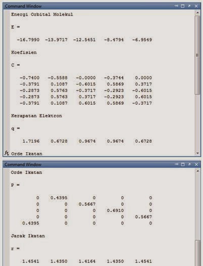
here some sample I get,


- Sea current data used here is NetCDF file, for example I use current data from Ocean Surface Current Analyses - Real time (OSCAR) NOAA which can be downloaded here.
- Download GSHHS shapefile here as a coastline.
- Open Matlab and use this script.
clc
clear all
close all
uc=ncgeodataset('arusindian.nc');
lat=uc.data('lat');
lon=uc.data('lon');
for i=find(lon>180):length(lon)
lon(i)=lon(i)-360;
end
time=uc.time('time');%result 754324
tgl=datestr(time);
north = max(lat); % batas utara
south = min(lat); % batas selatan
west = min(lon); % batas barat
east = max(lon); % batas timur
s=gshhs('gshhs_l.b',[double(south) double(north)], [double(west) double(east)]);
arus_u=uc{'u'}(1,1,:,:);
arus_u=reshape(arus_u,size(arus_u,3),size(arus_u,4));
arus_v=uc{'v'}(1,1,:,:);
arus_v=reshape(arus_v,size(arus_v,3),size(arus_v,4));
dx=0.1;
[lon_r,lat_r]=meshgrid(west:dx:east+2,south:dx:north+2);
ucur=interp2(lon,lat,arus_u,lon_r,lat_r,'cubic');
vcur=interp2(lon,lat,arus_v,lon_r,lat_r,'cubic');
da=1.7;
[lon_a,lat_a]=meshgrid(west:da:east,south:da:north);
ucura=interp2(lon,lat,arus_u,lon_a,lat_a,'cubic');
vcura=interp2(lon,lat,arus_v,lon_a,lat_a,'cubic');
mag=sqrt(ucur.^2+vcur.^2);
quiver(lon_a,lat_a,ucura,vcura,'k','LineWidth',1.13);
hold on
pcolorjw(lon_r,lat_r,mag);
geoshow(s,'facecolor',[0 0 0]);
z=colorbar;
set(get(z,'ylabel'),'String','Speed (Knots)','fontweight','bold');
axis equal
axis([west east south north]);
caxis([0 1])
xlabel('Longitude','fontweight','bold');
ylabel('Latitude','fontweight','bold');
title(['Arus Muka Laut Pada ' tgl(1,:)],'fontweight','bold');
set(gcf,'renderer','zbuffer','paperpositionmode','auto');
here some sample I get,